The Extent Account

The SEEA EA includes as first core ecosystem account the Ecosystem Extent Account, or ‘extent account’. This account records the area covered by different ecosystem types. Ecosystem types, are for instance a deciduous forest, or a heathland.

There are several possibilities to classify ecosystems for extent accounting:

The IUCN Global Ecosystem Typology (IUCN GET) 2.0 (URL: 2020-037-En.pdf (iucn.org)) is a hierarchical classification system that, in its upper levels, defines ecosystems by their convergent ecological functions and, in its lower levels, distinguishes ecosystems with contrasting assemblages of species engaged in those functions. It is adopted in the SEEA EA guidelines as a reference classification. The IUCN typology comprises six hierarchical levels. The three upper levels – realms, functional biomes and ecosystem functional groups – classify ecosystems based on their functional characteristics (such as structural roles of foundation species, water regime, climatic regime or food web structure). The three lower levels of IUCN classification (which are not considered in the SEEA EA) - biogeographic ecotypes, global ecosystem types and sub-global ecosystem types - consider species assemblages living in the ecosystem types. The SEEA states in para 3.55: “It is recommended that existing national ecosystem classification schemes be used for ecosystem accounting wherever possible. Generally, such classification schemes will provide detailed descriptions and classes that incorporate specific local ecological knowledge. Cross-referencing of units to the SEEA EA reference classification, the IUCN Global Ecosystem Typology, will enable national level accounts to be scaled up and compared between countries. Where specific national ecosystem types have been identified that do not translate directly to the SEEA EA reference classification, local ecological expertise should be applied to determine the most appropriate cross-referencing.”. Furthermore, SEEA EA (paragraph 3.65) states “It is expected that for the purposes of international comparison, the reporting of data at the EFG level (level 3) would be appropriate”.

However, at national level, country level ecosystem classifications may be more appropriate. National schemes are most suited to the ecosystem types encountered in the country. A cross-walk with the IUCN GET may be developed for national reporting.

Furthermore, in the EU, a specific ecosystem typology has been developed, as a draft for testing, in support of ecosystem accounting in the EU (By Eurostat). This typology is now being tested and will be made available through the EU INCA platform. In its current set-up it counts three distinctive levels, with level 1 an elaborated version of the earlier MAES classification of ecosystems for Europe.

Like all accounts, the extent account comprises a map and an accounting table, which records ecosystem types in a given year, and, where multiple years of spatial data are available, changes in area from one reporting year (accounting period) to the next. Since extent accounts build upon ecosystem type maps, it has become common practice to develop the account for a specific year (reflecting ecosystem cover through the year, including for example annual crops growing during the summer period), rather than establish the ecosystem cover on the 1st of January or 31st of December of a given year. Furthermore, extent accounting normally includes a change matrix, that shows which ecosystem types were converted in which other ecosystem types, from one year to the next.



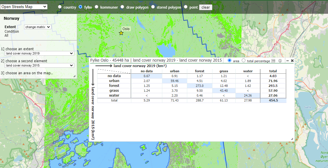
Example 1 of an extent account, the change matrix for Oslo, 2015 to 2019

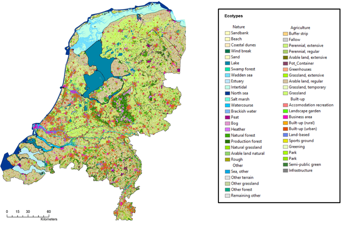
Example 2 of an extent account: ecosystem type map of the Netherlands (2018)


Netherlands ecosystem types map

The Condition Account

The ecosystem condition account presents biophysical information on the state or health of ecosystems. This is done using a variety of ecosystem condition indicators, that may address: vegetation (e.g. standing stock of biomass), soil (e.g. acidity or soil organic matter), or water (e.g. total nitrogen concentration, or presence of water quality indicator species).

A major challenge is comparing ecosystem condition indicators: if one indicator shows improvement of ecosystem condition, and another degradation, what does this say about overall ecosystem condition? Moreover, it is sometimes difficult to define when a change in an indicator constitutes an improvement, or indicates degradation. Often, a natural ecosystem condition (e.g., Ph, or standing stock, or species diversity) is used as ecosystem condition reference level against which to compare trends in individual indicators, however such reference levels are sometimes hard to develop (e.g. when ecosystems have been converted from their natural state long time ago) and this approach is currently being further developed.

In case reference levels are hard to establish an alternative is to present ecosystem condition indicators without reference level, as was done in the Netherlands ecosystem accounts, see the example below.


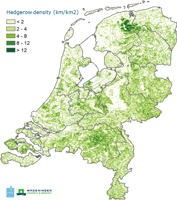
Example 3. Condition account map of hedgerow density, an indicator for landscape attractiveness and relevant for biodiversity conservation.




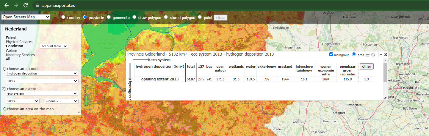
Example 4. Hydrogen deposition in Gelderland in 2013

The physical ecosystem services supply and use account

The biophysical ecosystem service supply and use account records the flows of ecosystem services from ecosystems to society, in physical terms. The flow comprises the accumulation of a service in a given accounting period, usually taken as one year (but in principle accounts
can also be compiled on a quarterly on monthly basis). Each service needs to be carefully defined to represent the contribution of the ecosystem to economic activity. Proposals for indicators can be found in the SEEA EA, insert URL, see: eea.un.org). It is noted that in ecosystem accounting, supply of an ecosystem service equals use (both in physical and in monetary terms). Supply of the service is by the ecosystem (to be specified by ecosystem type) and use is in the economy, and can be specified by economic sector.

Not all ecosystem services are straightforward to define. For example, the definition of ‘crop production’ is quite challenging, since a wide range of biophysical processes contribute to facilitating crop production by farmers (e.g. nutrient storage and release by soil particles,
water holding capacity, and earth worm activity). In line with the SEEA EA it is recognised that these individual processes cannot all be analysed and therefore, as a proxy indicator, the
amount of crop yields was used as physical indicator (recognising that crop production is as much a function of ecosystem properties and processes as it reflects farmers’ activities). The consequence of this approach is that the physical ecosystem services account shows higher
physical output for the crop provisioning service (but generally not for other services) in intensive versus extensive agricultural systems, reflecting the use of higher quantities of fertilisers and pesticides, among others, in intensive systems. In the monetary ecosystem services account, however, the costs of fertilisers, pesticides and labour inputs are considered, thereby showing a more accurate reflection of the contribution of the ecosystem to agriculture compared to the physical account.


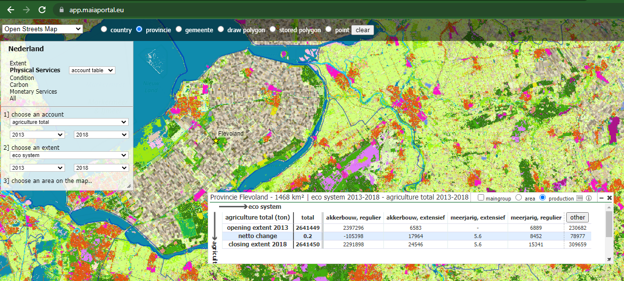
Example 5. account table for total agriculture in Flevoland (2013-2018), see the manual on how to make these tables in the MAIA Analitical Tool.

The monetary ecosystem services supply and use account

In the SEEA EA, monetary valuation is conducted in a manner that is aligned with information in the standard national accounts ((see: url: System of National Accounts). This enables comparison of the supply and use of ecosystem services with the production and consumption of other goods and services and supports the use of ecosystem information in standard economic modelling and productivity analysis. A key concept in the SNA and the SEEA is that of ‘exchange values’ – i.e. the values at which goods, services, labour or assets are in fact exchanged or else could be exchanged for cash (currency or transferable deposits). For goods and services traded in a market, the exchange value reflects market prices. Market prices for transactions are defined in the SNA as amounts of money that willing buyers pay to acquire something from willing sellers; the exchanges are made between independent parties and on the basis of commercial considerations only. In this context, a market price should not necessarily be construed as equivalent to a free market price; that is, a market transaction should not be interpreted as occurring exclusively in a purely competitive market situation.

Importantly, valuation approaches consistent with the SNA exclude consumer surplus, but include producer surplus and costs of production. The SNA includes specific value indicators such as gross and net value added and operating surplus. In the SEEA EEA Technical Recommendations, it is explained how these value indicators can be applied to and extended for the purpose of ecosystem accounting (URL Technical Recommendations in Support of the SEEA-EEA | System of Environmental Economic Accounting). This difference in scope is a fundamental difference between valuation approaches applied in SEEA and values commonly used in environmental cost-benefit analysis (e.g. URL Valuing Ecosystem Services: Toward Better Environmental Decision-Making |The National Academies Press)


In the monetary ecosystem services supply and use account, therefore, ecosystem services are valued based on exchange values. Potentially applicable methods for valuation are:

1. rent-based approaches (e.g. rent paid for farmland can be used to value to crop provisioning service)
2. replacement cost method (in case it can be assumed that the service would indeed be replaced if lost
3. avoided damage cost method (if it can be assumed that the service will NOT be replaced
4. hedonic pricing (to disentangle the environmental contribution to a property traded in a market
5. consumer expenditure: in particular for the tourism and recreation service
6. simulated exchange value method (SEV) (in case other methods are not applicable, and there is no (substitute) market that can be consider to reveal a price for the ecosystem service. In SEV, a price established based on a demand curve for the ecosystem service to be valued -> based on this demand curve the price is assessed that, if users were to be charged for the service, would bring the highest profit to the ecosystem. This valuation approach is consistent with the valuation principles of the SNA and can be used to value ecosystem services harvested in a common pool, open access situation, for instance.

Ecosystem asset account

The value of ecosystem assets can be derived using the Net Present Value (NPV) approach. Applying a NPV approach requires assessing the present and expected future flow of all ecosystem services, and aggregating the NPV of each service flow. Changes in future flows of service, for instance due to ecosystem degradation or depletion of resources (e.g., timber) due to overharvesting need to be considered by reducing flows of ecosystem services supply in future years. Often, in the absence of data, it is assumed that all flows remain constant, i.e. that there is no degradation resulting in a decrease in ecosystem service flow in the coming decades.
Furthermore, it is often assumed that there are no changes in prices for ecosystem services (which, with increasing ecosystem capital scarcity and therefore potential upward pressure on such prices, may lead to an underestimate of the value of ecosystems). In the future, these assumptions need to be further tested, and potentially more realistic assumptions may be applied in ecosystem accounting.

Calculating the asset value requires making an assumption on asset life and selecting a discount rate. Asset life is often (e.g., as in the case of the UK and the NLs ecosystem accounts) assumed to be 100 years – i.e. it is assumed that the ecosystem ‘produces’ ecosystem services for a period of 100 years. This period is somewhat arbitrary, but values provided after 100 years do not contribute much to the Net Present Value because of the discount rate applied. A key element in assessing NPV is the discount rate. For public investment analysis, often a lower discount rate is used than for discounting private investment options. Often, a discount rate of 2 or 3% is used in ecosystem accounting, in line with rates used in public sector decision making. The case could be made that for ecosystems, due to increasing scarcity and limited substitution possibilities, a discount rate of 2 percent would be more appropriate.

Thematic accounts

The Biodiversity account

Guidance for Biodiversity Accounting is provided by the Convention on Biological Diversity (CBD), the Technical Recommendations ford SEEA EEA, and the 2021 SEEA EA. The CBD, in its 2010 global biodiversity targets proposes a series of sets of indicators of which the ones for status and trends of the components of biological diversity are of direct relevance for the SEEA
EA biodiversity account. Indicators proposed include

1. trends in extent of selected ecosystems,
2. trends in abundance and distribution of selected species,
3. trend in status of threatened species and
4. changes in genetic diversity. Additional groups of indicators for e.g. threats to biodiversity, ecosystem integrity, and accessibility are more appropriately covered by the SEEA EA Condition account.

These indicators are comparable with indicators mentioned in the SEEA EEA technical guidance document on experimental biodiversity accounting (URL: Guidance on experimental biodiversity accounting using the SEEA-EEA framework - UNEP-WCMC), which focusses on 3 tiers, ranked by increasing information requirements:

1. ecosystem extent
2. species richness distributions
3. species abundance.

It is noted that a broad range of indicators within each of these three groups can be selected, e.g. focusing on different types of species (birds, plants, insects, etc.) or considering all species or only threatened and/or endemic species. The challenge in biodiversity accounting is to define a mix of indicators that captures main elements of a country’s (or area’s) biodiversity, is policy relevant, and is measurable given data availability (with trends, i.e. multiple years of data of particular relevance).

The Carbon account

The carbon account provides a comprehensive overview of all relevant carbon stocks and flows, and other relevant greenhouse gasses related to ecosystems (N2O and CH4, in particular) in ecosystems. It may cover carbon and other GHG stocks and flows in the reservoirs ‘biocarbon’
(organic carbon in soils and biomass), ‘geo-carbon’ (carbon in the lithosphere), and atmospheric carbon and carbon in the economy; or focus on carbon in ecosystems (above ground and below ground) only.

The Ocean account

The Ocean account is one of four thematic accounts present in the 2021 SEEA EA, but not in the original 2012 SEEA EEA framework. It has been added in recognition of the need to develop a specific approach for oceans that allows dealing with the three-dimensional structure of oceans – in addition to geographic coordinates, oceans cover benthic up to pelagic ecosystems, that generally are very different in terms of species composition, food webs, and human use. Several countries have produced pilot ocean ecosystem accounts that include extent indicators (e.g. area covered by specific ecosystem types), condition (related to water quality and/or biodiversity), services (e.g., fisheries, tourism, sand mining, etc.) and asset values.

The Urban ecosystem account

As with the Ocean account, the Urban ecosystem account was added to the 2021 SEEA EA. It allows zooming in on the extent and condition of ecosystems, and the services they supply, in urban areas. Typically, the urban ecosystem account has a higher resolution than a national level ecosystem account, and it may focus on different ecosystems. For example, local climate regulation (cooling of cities due to the presence of vegetation) may be a relevant service in urban ecosystem accounts, whereas carbon sequestration may be less relevant in cities with limited green space. An important issue is how the territory of the urban ecosystem account is defined, with one option being Functional Urban Areas (i.e. cities and the surrounding landscape where people go for recreation or where commuters live). In case such a broad area is selected, clearly, carbon sequestration is more relevant compared to a situation where a narrow, municipal boundary of a city is chosen.